Getting a depth map out of blender is a little akward, but possible. The method that is usually recommended isn't entirely correct though. So let's take a look at it and find out what's wrong.

The Usual Method

You can get the depth from Blender via the Compositor, for artistic purposes. However, it's not obvious, how you could get the raw depth values (e.g. in a numpy-array). The usual approach goes like this:

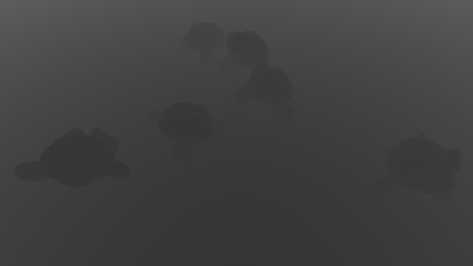
The Map Range is necessary in order to be able to view the depth as an image (rgb ranges from 0..1 or 0..255 respectively). Usually, you take your near- and far-plane of the camera as the input range. Resulting in the following map (access and save via Image Editor):

Now to get the actual numeric values, you need to access the image output from the Viewer Node:

import bpy
import numpy as np

depth = np.asarray(bpy.data.images["Viewer Node"].pixels)
depth = np.reshape(depth, (540, 960, 4))
depth = depth[:, :, 0]
depth = np.flipud(depth)
depth = reverse_mapping(depth)

np.save("/tmp/depth.npy", depth)

Note that reverse_mapping is just a placeholder for a function that reverses the mapping you had to do in order to fit the depth data into the image. Which btw is stored linearly, independent of blenders output format, as long as it is not written to file:

Image data-blocks will always store float buffers in memory in the scene linear color space

Doing the above, we receive the following:

%config InlineBackend.figure_formats = ['svg']
import matplotlib.pyplot as plt
import numpy as np

dist_monk = np.load("depth_monk.npy")

plt.imshow(dist_monk, vmin=0, vmax=15)
plt.show()

Where's the Catch?

Now you might be content, but be aware! What you have in front of you is not a depth map in the actual sense of the word. That is, it actually is a distance map.

To clarify the difference: Imagine you're looking straight at a flat wall. What depth map do you expect?

A flat one, right? Uniform color, representing a uniform distance from the image plane. Now let's look at what happens if we point the Blender camera at a wall:

dist_wall = np.load("depth_wall.npy")

plt.imshow(dist_wall, vmin=4, vmax=7)
plt.show()

How about that.. What does this mean?

It means, that we're not measuring the distance from the image plane, but instead the distance from the camera position. Which is strange, since the z-vector for each pixel is different. Each pixel gets measured by the distance along the view-ray of the camera.

There is no common base coordinate frame for the pixels in the image.

To make this usable as an actual depth image – that encodes everything relative to the image coordinate frame, we need to project each view-ray back onto the image z-axis.

Turning the Distance Image into a Depth Image

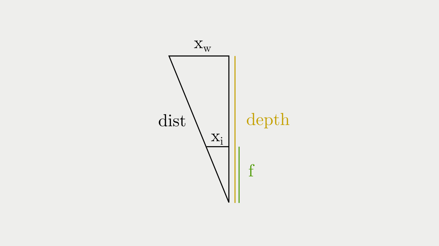
So, how do we get the depth from the distance? Let's sketch the pinhole camera model for this scenario:

So, we just need to pythagoras our dist into a depth.

$depth^2 + x_w^2 + y_w^2 = dist^2$

However, since $x$ and $y$ are in image units (px) but our depth in world units (mm or similar), we need to convert the two into each other.

This is what $x_w$ and $y_w$ stand for. $x$ and $y$ in world units. We can get them using our knowledge of similar triangles (with $x_i$ being x in image units and $f$ being the focal length of the camera):

$\frac{x_w [mm]}{depth [mm]} = \frac{x_i [px]}{f [px]}$

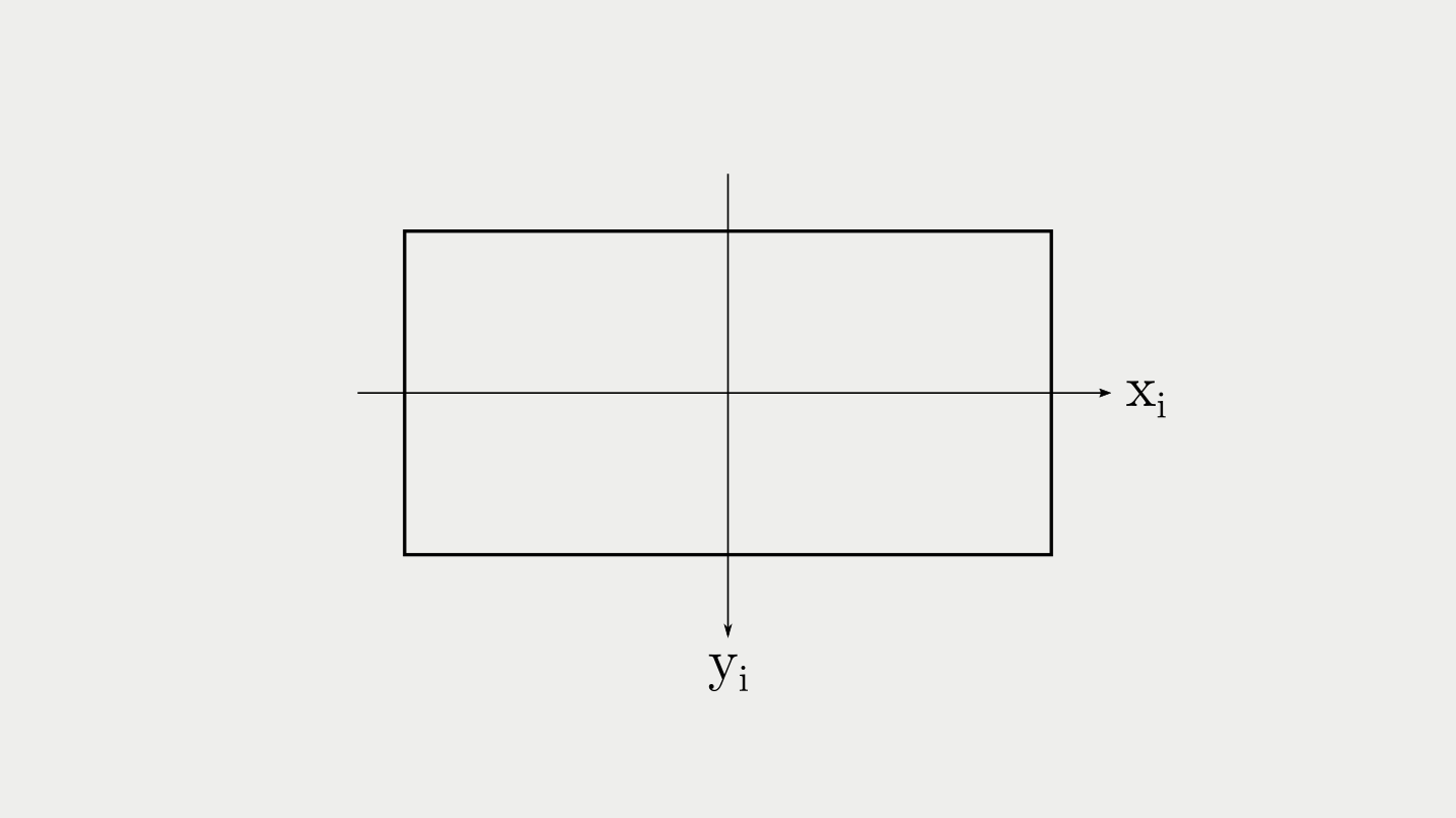
With $x_i$ and $y_i$ being in the following frame:

Combining both equations, we get the following formula for the depth at a certain pixel:

$depth = \sqrt{\frac{dist^2}{ \frac{x_i^2 + y_i^2}{f^2} + 1 }}$

For this to work, our focal length has to be in pixels, as has to be our sensor size. This is, because we need a link between the pixels and the world units.

def dist2depth_img(dist_img, focal=500):
    img_width = dist_img.shape[1]
    img_height = dist_img.shape[0]

    # Get x_i and y_i (distances from optical center)
    cx = img_width // 2
    cy = img_height // 2

    xs = np.arange(img_width) - cx
    ys = np.arange(img_height) - cy
    xis, yis = np.meshgrid(xs, ys)

    depth = np.sqrt(
        dist_img ** 2 / (
            (xis ** 2 + yis ** 2) / (focal ** 2) + 1
        )
    )

    return depth

depth_wall = dist2depth_img(dist_wall)

plt.imshow(depth_wall, vmin=4, vmax=7)
plt.show()

Awesome, a flat wall. Our correction is working! Now let's go back to the Suzannes:

depth_monk = dist2depth_img(dist_monk)

plt.imshow(depth_monk, vmin=0, vmax=15)
plt.show()

Looks good.. I fixed the scale in these plots, so that the colors represent the same depth. However, the difference is more striking if you let matplotlib exploit each images own data-range (in all of viridis' glory):

You can clearly see the spherical correction that has taken place (no wonder since we divide the distance-map by what is basically a circle-equation).

This depth map can now be used with standard reprojection workflows to generate a point cloud of the scene.

Cheers,

max